

Buckets and time
Counters, gauges and timers do not store what you wrote. They store a summary of a time window, and that window is called a bucket.
This page explains what a bucket actually is once it reaches your database, why summarising before you store is worth doing, what it costs you, and how to pick the two settings that control it.
Why buckets exist at all
Say you run an API that serves 2,000 requests a second, and you want to answer "how many requests per minute did each route get last Tuesday".
The obvious approach is one database row per request.
INSERT INTO requests_raw (ts, route, status) VALUES (now(), '/checkout', 200);That gives you a perfect record and a problem. At 2,000 a second you are writing 172.8 million rows a day to answer a question about a few thousand numbers. Every time anyone opens the dashboard, the database reads all of those rows back and adds them up again.
The alternative is to add them up as they happen, in memory, and write only the totals. Assume the API has 40 routes and four status classes, so there are 160 possible combinations, and one minute buckets.
| One row per request | One row per minute | |
|---|---|---|
| Rows written per day | 172,800,000 | up to 230,400 |
| Bytes per day, before compression | about 35 GB | about 14 MB |
| Rows read to chart one day | 172,800,000 | 230,400 |
| Insert calls per day | millions | 1,440 |
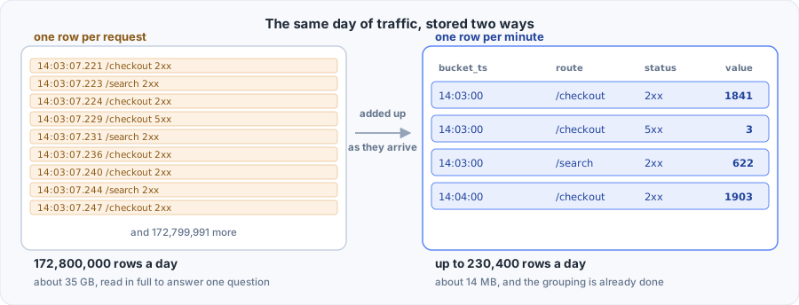
Same question, same answer, about 750 times less of everything. That is what a bucket buys, and MetricHouse exists to do the adding up correctly.
This is not a replacement for keeping the detail
A bucket answers "how many". It cannot answer "which user" or "what was the request id", because that information was added away. When you need the detail, use an event, which keeps every record whole. Most systems want both, and the two work together.
A bucket is a GROUP BY you did in advance
The clearest way to think about a bucket row is as a query result that was computed before anyone asked.
Here is the query your database would have to run over raw rows:
SELECT
  date_trunc('minute', ts) AS bucket_ts,
  route,
  status,
  count(*)                 AS value
FROM requests_raw
GROUP BY 1, 2, 3;
MetricHouse runs exactly that grouping in memory, as the requests arrive, and writes the result. The correspondence is one to one:
| In the query | In the row MetricHouse gives you | Comes from |
|---|---|---|
date_trunc('minute', ts) | bucket_ts | resolution: '1m' |
route, status | route, status | your dims |
count(*) | value | the add() calls |
So this declaration:
const requests = counter('requests', {
  dims: { route: str(), status: oneOf(['2xx', '4xx', '5xx']) },
  resolution: '1m',
  flush: '5m',
  write: async (rows) => db.insert(rows),
})

requests.add({ route: '/checkout', status: '2xx' })
produces rows that look like this:
id                                bucket_ts            route      status  value
4f2c18a6e1d9b0c73a5e8f21b6d40c99  2026-09-17 14:03:00  /checkout  2xx     1841
a91e5b7c2d380f4419ce6a05d7b2f318  2026-09-17 14:03:00  /checkout  5xx     3
7d10c4b9e5a2f68301bd97e4c2a5f0b6  2026-09-17 14:03:00  /search    2xx     622
4b8e10f3a75c29d6e0148bca39f5d720  2026-09-17 14:04:00  /checkout  2xx     1903
Read one row as a sentence: between 14:03:00 and 14:04:00, /checkout returned a 2xx status 1,841 times.
Three things follow from that, and they are worth knowing before you choose a resolution.
One row per combination, per window. The natural key of the table is bucket_ts plus every dimension. That is what naturalKey() returns, and it is what your table should treat as unique.
A row only exists where something happened. If no request hit /search during 14:03, there is no row for it. The table is sparse, which keeps it small, and it means a chart gets a gap rather than a zero. Fill those in when you query if your chart needs them.
The window is half open. A row stamped 14:03:00 covers 14:03:00.000 up to but not including 14:04:00.000. A request at exactly 14:04:00.000 belongs to the next row. Every range in MetricHouse works this way, so counts never double up at a boundary.
Bucket rows still add up
This is the property that makes bucketing safe rather than lossy, and it is the reason the library stores what it stores.
A minute table can answer hourly, daily and monthly questions, because summing sums gives you the right sum:
-- One minute rows, rolled up to hours. No loss, no approximation.
SELECT
  date_trunc('hour', bucket_ts) AS hour,
  route,
  sum(value)                    AS requests
FROM requests
GROUP BY 1, 2;
The same holds for a gauge and a timer, which is why they store sum and count rather than an average. min takes the smallest, max takes the largest, sum and count add, and the average is sum(sum) / sum(count) whenever you want it. An average stored per bucket could not be merged, because the mean of two means is only the real mean when both windows saw the same number of observations.
So the rule is simple:
You can always make a bucket coarser later. You can never make it finer.
Resolution is the floor on every question you will ever ask of that table.
What you give up
Being honest about the trade matters more than the benefits, because the benefits are obvious and the costs are the part people discover later.
You cannot go below the resolution. A '1m' counter can never tell you whether those 1,841 requests arrived evenly or all in one second. If you later decide you need that, you change the setting and start collecting it, but the history stays at one minute.
You cannot ask about individuals. The counter above knows 1,841 requests happened. It does not know who made them. Put anything unique per occurrence on an event instead.
You cannot add a dimension retroactively. The grouping happened before the row was written, so a dimension you did not declare was never captured. Adding one later affects new rows only, and reordering the ones you have is a breaking change. dims covers both.
Changing resolution splits your history. Rows already shipped keep their old boundaries, and so do windows still in the driver when you deploy: they ship with the boundaries they were written with. Every write made after the deploy lands on the new grid. A chart that reads raw bucket_ts values will see the granularity change at the point you made the switch, while any query that groups to something coarser than both resolutions reads old and new rows alike, which is almost every query. Flushing before you deploy, as Changing a schema with data in storage describes, keeps the switch to a single point in time. A write for a window the old resolution already shipped is moved to the first window of the new resolution at or past that point. Going from one minute to five, a write for 12:05 after 12:07 has shipped lands in 12:10 (A write that misses its window).
Where the boundaries are
A bucket is resolution wide, and the boundaries are measured from the Unix epoch rather than from when your process started. A one minute bucket always starts on the minute. A ten second bucket always starts on a multiple of ten seconds.
That sounds like a detail and is actually the reason the whole thing works across more than one server. Two processes that started minutes apart still agree exactly where every boundary is, with no coordination between them, so they contribute to the same row rather than to two rows that have to be reconciled later. It also means your bucket_ts values line up with any other time series you already have.
Three settings, three owners
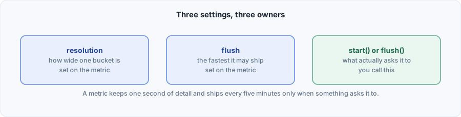
| Setting | What it controls | Who decides |
|---|---|---|
resolution | How wide one bucket is, which is how much detail you keep | The metric |
flush | The fastest this metric is allowed to ship | The metric |
start() or flush() | What actually asks it to ship | You |
Keeping these apart is the useful part. A metric can hold one second of detail and still only talk to your database every five minutes.
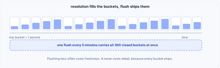
Shipping less often costs freshness. It never costs detail, because a flush takes every finished bucket, not just the most recent one.
Try it
Try it: resolution inside flush
The declaration these settings produce
counter('requests', {
  resolution: '1s',
  flush: '5m',
  write: async (rows) => db.insert(rows),
})
Your sink receives id, bucket_ts, …dims, value, one row per combination per bucket.
Press Run the clock to watch a window fill and ship. Then widen flush without touching resolution, and notice that the rows per day never move.
What each setting actually changes
This is the table to come back to. Almost every question about tuning is answered by one row of it.
resolution | flush | |
|---|---|---|
| Rows stored per day | sets it | no effect |
| Detail you can query later | sets it | no effect |
| How stale your database is | no effect | sets it |
| Number of insert calls | no effect | sets it |
| Rows carried by one insert | affects it | affects it |
| Memory held in the driver | affects it | affects it |
| Data at risk if the process dies | no effect | sets it |
The two that share a row work the same way in both cases:
rows per insert  =  (flush / resolution) × active combinations
cells in driver  =  (flush / resolution) × active combinations
"Active" means combinations that actually saw a write. A combination nothing touched costs nothing.
Finer resolution or a longer cadence both mean more buckets waiting, so both raise the memory a driver holds and the size of one insert.
Resolution has to divide flush
If resolution does not divide flush evenly, a shipment would cut a bucket in half. MetricHouse refuses that at declaration time rather than letting you find out from a wrong number later.
counter('ok', { resolution: '1s', flush: '5m', write })    // 300 whole buckets
counter('ok', { resolution: '10s', flush: '1m', write })   // 6 whole buckets

counter('bad', { resolution: '7s', flush: '1m', write })
// Error: bad: resolution 7s does not divide flush 1m evenly
Choosing a resolution
Ask one question: what is the shortest event you need to be able to see?
A spike that lasts ten seconds is still visible in a one minute bucket, as a bump. What you lose is the ability to tell a ten second surge at six times the rate apart from a full minute at the normal rate. If that distinction matters for the decision you are making, you need a resolution at or below the length of the thing you are looking for.
Then check the cost:
rows per day = (86,400 / resolution in seconds) × combinations that saw traffic| Resolution | Rows per combination per day | Reasonable for |
|---|---|---|
'1s' | 86,400 | Rate limits, incident timelines, money |
'10s' | 8,640 | Request and error rates on a busy service |
'1m' | 1,440 | Most application metrics. Start here |
'5m' | 288 | Business counts, slow moving numbers |
'1h' | 24 | Billing rollups, daily reporting |
Multiply by your combination count to get the real number. A '1s' counter with 50 combinations is about 4.3 million rows a day, which ClickHouse will not notice and Postgres will.
Two practical notes:
- Start coarse. Going from
'1m'to'10s'later is a one line change, and old rows stay valid because they carry their own timestamps. - The floor is permanent. You cannot recover detail you never wrote, so if a metric carries money or feeds an alert that has to fire quickly, spend the rows up front.
Choosing a flush
flush does not change what you store. It changes when you store it, so pick it from four questions.
How stale may the database be? A '5m' cadence means your dashboard is up to five minutes behind. That is usually fine, because a live read answers the "right now" question without touching the database at all. See Reading live data.
How often do you want to write? A '1m' cadence is 1,440 inserts a day per metric. A '5m' cadence is 288. If you have forty metrics on a shared database, that difference is real.
How much data can you afford to lose? Everything unflushed lives in the driver. With ioredis() that survives a crash, so the cadence only affects freshness. With memory() it does not, and the cadence is exactly how much data a crash costs you.
How large may one insert be? A long cadence with a fine resolution produces big batches. Five minutes of one second buckets across 500 combinations is up to 150,000 rows in one call. Chunk it in your sink, or shorten the cadence.
| Flush | Inserts per day | Suits |
|---|---|---|
'10s' | 8,640 | A dashboard that has to be nearly live off the database |
'1m' | 1,440 | The common default |
'5m' | 288 | Most business metrics |
'15m' | 96 | Slow moving numbers, expensive write paths |
'1h' | 24 | Archival rollups |
Choosing both: some starting points
| Situation | resolution | flush | Why |
|---|---|---|---|
| HTTP request and error rates | '10s' | '1m' | Enough detail to see a spike, one insert a minute |
| Business counts: signups, orders | '1m' | '5m' | Nobody charts these per second |
| Money taken and refunded | '1s' | '5m' | Reconcile an incident by the second, ship in batches |
| Rate limits and quotas | '1s' | '1m' | The live read does the work, the table is the record |
| Queue depth and system health | '1m' | '1m' | Sampled every ten seconds, so a minute holds six values |
| Device readings from the field | '1m' | '15m' | Devices report slowly, so batch the writes |
| Billing rollups | '1h' | '1h' | 24 rows a day per customer |
If you are not sure, start at resolution: '1m' and flush: '1m', watch the row count for a week, and adjust. Both are configuration changes, and neither invalidates what you already stored.
Grace: letting a late write land
A bucket does not become eligible for shipping the instant it ends. It waits for a short grace period first.
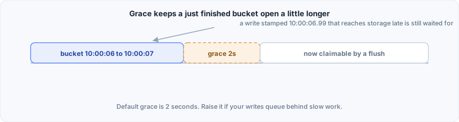
A write is stamped with its window at the moment you call add(), set() or end(). Reaching storage takes a little longer. On Redis it is a network round trip, and a busy process can hold a write in its queue for a while before it goes out. So a write stamped 10:00:06.990 can reach Redis at 10:00:07.050, after its window has ended. Grace holds the window back from the flush until writes like that have had time to arrive.
Grace does not move a write into an earlier window. A request that starts at 10:00:06.980 and calls add() at 10:00:07.010 is counted in the 10:00:07 window, because that is when it was recorded. A timer works the same way: a timing lands in the window its end() is called in.
The default is 2 seconds. Raise it if your writes queue behind slow work, or if your servers' clocks disagree by more than that.
const slowJobs = counter('slow_jobs', {
  resolution: '1m',
  flush: '5m',
  grace: '30s',        // this queue can take a while to reach Redis
  write: async (rows) => db.insert(rows),
})
A write that misses its window
Sometimes a write arrives after its window has already been claimed by a flush: grace was too short, or the server that made it has a clock running behind. That write is moved forward into the first window of its own resolution at or past the watermark, and it ships with that window.
The driver keeps track of this with a watermark per metric: every window below it has been claimed at least once. A write aimed below the watermark lands on the first window of the metric's own resolution at or past it. The watermark is a timestamp and may fall between two of those windows, for instance when the resolution has changed since the flush that set it, and the write still lands on a window the metric's rows can name.
The total stays exact, and every row id still ships with one final value. The cost is that the write is counted a window or two later than it happened. A table that treats id as unique handles this with no special work, whether it keeps the first row per id or the newest.
A flush raises the watermark to the point it claimed up to, but no further than the newest window that held any data when it claimed. Windows beyond that one were empty, so nothing shipped for them, and a write that arrives for one of them later keeps its own window. This limit matters when a single flush runs on a clock that is far ahead, say by two days. Without it, every write for the next two days would be moved into one window, which no flush could claim until the clock caught up.
The same rule has a consequence when a server's clock runs ahead. A flusher on that server claims windows that are still open everywhere else, and the writes of correctly clocked servers for those windows move forward to the fast server's idea of now. Totals stay exact, but those writes land in windows up to the size of the skew ahead of their own. Keep your servers on NTP.
A clock that steps backwards, for instance after an NTP correction, can leave the watermark ahead of the clock. A write made then is moved to the first window past the watermark, which is ahead of the clock as well. Here is what happens to it:
current()reads the window a write made now lands in, so the moved write counts in the open total.snapshot({ complete: false })includes it. A complete snapshot leaves it out, the same way it leaves out the open window.- An ordinary flush ships it once the clock has passed the end of that window plus grace, like any other window.
- A final flush on a driver whose storage ends with the process, such as
memory(), also claims every window ahead of the clock, and leaves only the window the clock is in. Sohouse.stop()ships these writes rather than losing them. The same applies to a write made before the clock stepped back, whose window is now ahead of the clock too. - On a driver whose storage outlives the process, such as
ioredis(), a final flush leaves them in storage. The first flush whose clock has passed them ships them, from this process after a restart or from any other process.
A clock that steps backwards
When the watermark is not ahead of it, a server whose clock is corrected backwards writes into windows older than the ones it wrote to a moment before. For a counter, a gauge or a timer, that only counts the writes after the step in an earlier window.
A level is different, because it keeps one current value and decides which reading is newest by the window each was written in. A set() made after the step lands in an earlier window than the one made before it, so as far as the level can tell it is the older reading. It fills its own window and the empty windows after it, and the reading from before the step stays current. current() keeps returning that reading, and every flush keeps carrying it, until something writes to its window or a later one. With the clock only corrected by a second or two, the next write after the clock has caught up puts it right.
Flush is a minimum, not a schedule
The flush setting says how fast a metric is allowed to ship. It does not make anything happen.
setInterval(() => house.flush(), 10_000)That runs every 10 seconds. A metric with flush: '5m' still ships only every 5 minutes. The calls in between return a report saying it was skipped:
const report = await requests.flush()
// { buckets: 0, rows: 0, skipped: true, reason: 'cadence', nextEligibleInMs: 218000 }
Calling too often is harmless. Calling too rarely only delays delivery.
An empty flush does not use up the cadence
If a flush finds nothing to ship, the clock does not move forward. Otherwise an early empty flush would block the next real one for a full interval.
Working out a boundary yourself
Every metric reports its own resolution in milliseconds, so you can line live rows up with history from your database without guessing.
const res = requests.resolutionMs                  // 60000

const currentBucket = Math.floor(Date.now() / res) * res
const nextBoundary = currentBucket + res
Rows from snapshot() carry the same bucket_ts value your write function receives, so a chart can stitch the two together and know when it is looking at the same row twice. See Reading live data.